Building large scale data ingestion solutions for Azure SQL using Azure databricks - Part 1
Discover how to bulk insert million of rows into Azure SQL Hyperscale using Databricks
Source Code

With rise of big data, polyglot persistence and availability of cheaper storage technology it is becoming increasingly common to keep data into cheaper long term storage such as ADLS and load them into OLTP or OLAP databases as needed. In this 3 part blog series we will check out newly released Apache Spark Connector for SQL Server and Azure SQL (refered as Microsoft SQL Spark Connector) and use it to insert large amount of data into Azure SQL Hyperscale. We will also capture benchmarks and also discuss some common problems we faced and solutions to them.
In this first post we will see to use Microsoft SQL Spark Connector to bulk load data into Azure SQL from Azure Data Lake and how to optimize it even further. In the second part we will capture and compare benchmarks of bulk loading large dataset into different Azure SQL databases each having different indexing strategy. And in the final post we will discuss an issue with deadlocks (that we will face along this journey) and potential solultion. In each of the posts in this series I will mention what environment and dataset I have used and also share direct links to the scripts used.
So lets get started.
Getting started with Microsoft SQL Spark Connector
Microsoft SQL Spark Connector is an evolution of now deprecated Azure SQL Spark Connector. It provides hosts of different features to easily integrate with SQL Server and Azure SQL from spark. At the time of writing this blog, the connector is in active development and a release package is not yet published to maven repository. So in order to get it you can either download precompiled jar file from the releases tab in repository, or build the master branch locally. Once you have the jar file install it into your databricks cluster.
Environment
We will be using Azure Databricks with cluster configurations as following -
- Cluster Mode: Standard
- Databricks Runtime Version: 6.6 (includes Apache Spark 2.4.5, Scala 2.11)
- Workers: 2
- Worker Type: Standard_DS3_v2 (14.0 GB Memory, 4 Cores, 0.75 DBU)
- Driver Type: Standard_DS3_v2 (14.0 GB Memory, 4 Cores, 0.75 DBU)
Libraries installed in the cluster -
- Microsoft SQL Spark Connector (jar) - Built at c787e8f
- codetiming (PyPI) - Used to capture metrics
- altair - Used to display charts
Azure SQL Server Hyperscale configured at 2vCore and 0 replicas. In this post we will be using a single database which has tables as per this SQL DDL script.
Azure Data Lake Gen 2 contains parquet files for the dataset we use which is then mounted on Databricks.
Dataset
We will be using 1 TB TPC-DS dataset v2.13.0rc1 for this blog series. Due to licensing restriction TPC-DS tool is not included the repo. However the toolkit is free to download here. However I did include a subset of SQL DDL statements for creating tables here that we use in this blog.
In this post we will be focusing on only 3 tables - store, store_returns and store_sales. As the name suggests store_sales and store_returns contains items sold or returned for different stores. For more information about the dataset refer to the specification document available in the TPC-DS toolkit.
There are no foreign key in the tables so Surrogate Key of store (s_store_sk) will be used to query and group results from store_sales (ss_store_sk) and store_returns (sr_store_sk).
This dataset was already available in my Azure SQL database and is then exported as parquet files using export notebook. In case you have the dataset as text files you can modify the export notebook accordingly.
Notice in the above output the store_sales dataset is partitioned on ss_store_sk. This partitioning strategy works for us as we will be filtering on ss_store_sk and only work with few of the stores. This will also set us up for an issue that we will face later. The same partitioning strategy is used for store_returns as well.
Bulk Loading data into Azure SQL Database
Our use case will be to load sales and returns for a particular store into Azure SQL database having row store indexes (Primary Key) on table. This means we will have to load data for each store from store table and all its associated sales and returns from store_sales and store_returns tables respectively. Surrogate key for store is what ties together all three tables.
To compare results we will capture the time it takes to insert records into each table. Therefore there are some boilerplate code that captures metrics which can be safely removed. Anything within # --- Capturing Metrics Start--- and # --- Capturing Metrics End--- block is used solely for capturing metrics and can be safely ignored. It does not have any impact on importing data into Azure SQL.
from codetiming import Timer
import pandas as pd
import os

path = "/mnt/adls/adls7dataset7benchmark/tpcds1tb/parquet/"
server_name = dbutils.secrets.get(scope = "kvbenchmark", key = "db-server-url")
username = dbutils.secrets.get(scope = "kvbenchmark", key = "db-username")
password = dbutils.secrets.get(scope = "kvbenchmark", key = "db-password")
schema = "dbo"

database_name = "noidx"
url = server_name + ";" + "databaseName=" + database_name + ";"
url
We start with importing relevant packages and getting secrets from our secret-store. In case you want to run the notebook for yourself, you will need to modify the above cell accordingly. I am using codetiming and pandas packages to capture metrics and is not needed for bulk importing itself.
from pyspark.sql.types import *

# List of table names
tables = ["store", "store_returns", "store_sales"]

# Map between table names and store surrogate key
table_storesk_map = {
  "store": "s_store_sk",
  "store_returns": "sr_store_sk",
  "store_sales": "ss_store_sk"
}

# Map between table names and schema
table_schema_map = {
  "store": [
    StructField("s_store_sk", IntegerType(), False),
    StructField("s_store_id", StringType(), False)
  ],
  "store_returns": [
    StructField("sr_item_sk", IntegerType(), False),
    StructField("sr_ticket_number", IntegerType(), False),
  ],
  "store_sales": [
    StructField("ss_item_sk", IntegerType(), False),
    StructField("ss_ticket_number", IntegerType(), False)
  ]
}

# List of stores that we use
stores = [row["ss_store_sk"] for row in spark.read.parquet(f"{path}/store_sales").filter("ss_store_sk IS NOT null").groupBy('ss_store_sk').count().orderBy('count', ascending=False).select("ss_store_sk").take(5)]
print(stores)
Next we initialize the tables and stores that we will use for importing into Azure SQL. table_schema_map is used to correct the schema to match that of database. This is a temporary workaround for issue #5. We will be bulk inserting data in store, store_sales and store_returns for 5 stores having highest number of records in store_sales. The count of records for each of the stores are as below. Overall we will be inserting ~30 million records into our database.
I have a method to truncate the tables that we are working with. This will make it easier for us to rerun any of tests without getting into trouble with duplicate Primary key.
def truncate_tables(url, username, password, tables):
  for table in tables:
    query = f"TRUNCATE TABLE {schema}.{table}"

    try:
      t = Timer(text=f"Tuncated table {table} in: {{:0.2f}}")
      t.start()
      driver_manager = spark._sc._gateway.jvm.java.sql.DriverManager
      con = driver_manager.getConnection(url, username, password)

      stmt = con.createStatement()
      stmt.executeUpdate(query)
      stmt.close()
      t.stop()
    except Exception as e:
      print(f"Failed to truncate table {table}", e)
def create_valid_table_schema(table_name, df_schema):
  return StructType([x if x.name not in map(lambda n: n.name, table_schema_map[table_name]) else next(filter(lambda f: f.name == x.name ,table_schema_map[table_name])) for x in df_schema])

def import_single_store(url, table_name, store_sk):
  try:
      df = spark.read.parquet(f"{path}/{table_name}")
      df = df.where(f"{table_storesk_map[table_name]} == {store_sk}")

      # Temporary workaround until Issue #5 gets fixed https://github.com/microsoft/sql-spark-connector/issues/5
      table_schema = create_valid_table_schema(table_name, df.schema)
      df = spark.createDataFrame(df.rdd, table_schema)

      t = Timer(text=f"Imported store {store_sk} into table {table_name} in : {{:0.2f}} ")
      t.start()

      df.write.format("com.microsoft.sqlserver.jdbc.spark") \
        .mode("append") \
        .option("url", url) \
        .option("dbtable", f"{schema}.{table_name}") \
        .option("user", username) \
        .option("password", password) \
        .option("tableLock", "false") \
        .option("batchsize", "100000") \
        .save()

      elapsed = t.stop()
      return elapsed
  except Exception as e:
    print(f"Failed to import {store_sk} into table {table_name}", e)
These two methods will be reused throught this blog. create_valid_table_schema method takes the schema of the parquet files and merges it with schema defined in table_schema_map. This is a temporary fix as discussed before.
import_single_store(url, table_name, store_sk) takes in the url of the database, the table name and the surrogate key (store_sk) of the store. It then reads the parquet file for the specified table filtered by store_sk. It corrects the schema, starts the timer and submits the insertion job to spark. The two parameters tableLock and batchsize are crucial.
tableLockor TABLOCK specifies that the acquired lock is applied at the table level. This option is helpful when inserting into Heap table.batchsizedescribes how many rows are committed at a time during the bulk operation. Play around with it to see how the system performs with different batch sizes. This option will become useful later when we bulk insert into a Clustered Columnstore Index (CCI).
def import_stores(url):
  for store_sk in stores:
      # -------- Capturing Metrics Start---------
      t = Timer(text=f"Imported store {store_sk} in : {{:0.2f}}")
      t.start()
      metrics_row = {'store_sk': f'{store_sk}'}
      # -------- Capturing Metrics End---------

      for table_name in table_storesk_map.keys():
        elapsed = import_single_store(url, table_name, store_sk)

        # -------- Capturing Metrics Start---------
        metrics_row[table_name] = elapsed

      elapsed = t.stop()
      metrics_row['Total'] = elapsed
      global metrics_seq_df
      metrics_seq_df = metrics_seq_df.append(metrics_row, ignore_index=True)
      # -------- Capturing Metrics End---------
import_stores loops over all stores and calls import_single_store for each table. Note that it waits for import_single_store to complete before continuing the loop and inserting into next table. Lets truncate the tables and run it to capture the reults.
truncate_tables(url, username, password, tables)
import_stores(url)
The import is going to succeed and the timings will be logged for each table.
There are two interesting things to notice when the jobs are running. First is that only one spark job runs at a time. This is because we are inserting into one table at a time and the spark will create only 1 job for each spark.write when inserting data into Azure SQL. This is important fact to keep in mind to optimize in future.
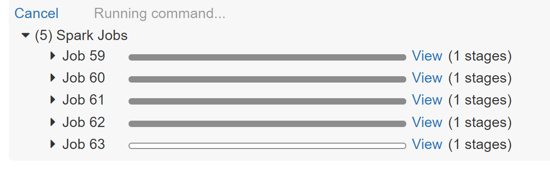
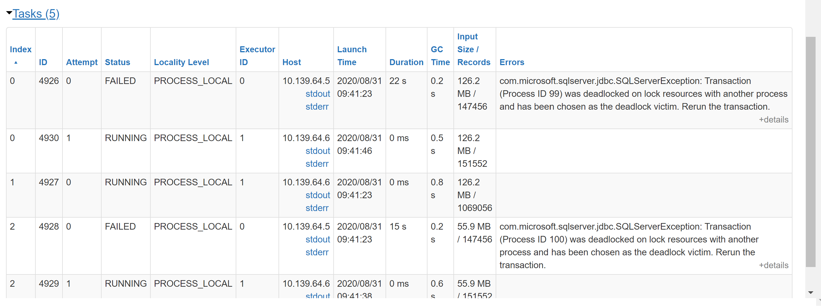
The second is a little tricky to find. If you check the stages of running job when it inserts into store_sales table in Spark UI you will notice some tasks will fail due to Deadlock.
com.microsoft.sqlserver.jdbc.SQLServerException: Transaction (Process ID 99) was deadlocked on lock resources with another process and has been chosen as the deadlock victim. Rerun the transaction.
Although these tasks failed the stage and job overall succeeded and this is due to retry mechanism within Databricks. This can be confirmed by counting number of records in database to perform a quick sanity check. We let it be for now as we will be discussing the root cause of deadlock and potential solutions in part 3 of this blog.
If you look at the timings it becomes obvious that overall time it took to insert all the data related to single store is sum of time it took to insert into each of the tables for that store. But can we do any better? Ususally in most system partially inserted data is not of use so we are delayed till the data is inserted for all related tables. So our next objective is to reduce the time it takes to insert all data for a single store. Wouldn't it be great if we can insert data for single store in all the tables concurrently?
Concurrently inserting data in all tables
To achieve this we will utilize Python's multithreading library to submit multiple spark jobs concurrently. As you would know, anything we write and execute through databricks notebook runs on executor. And when executor find statement related to spark, it submits the job to spark and spark then orchestrates its execution on the workers. The observation from above tells us that only single job (and single stage) is executing in our cluster at any moment. This means our cluster is woefully underutilized. Our plan is to submit multiple spark jobs to better utilize our cluster.
To make it work properly with python we have to set PYSPARK_PIN_THREAD environment variable in python and set it to true. You need to do this as part of cluster startup as setting it though Python's os module does not work. You can find more details about it in the doc. Note that as of yet this flag is not recommended in production. In case you want to perform such parallelization its better to use Scala. You can achieve same result in Scala using Futures and Awaits.
import threading

class myThread (threading.Thread):
   def __init__(self, table_name, store_sk):
      threading.Thread.__init__(self)
      self.table_name = table_name
      self.store_sk = store_sk

   def run(self):
      elapsed = import_single_store(url, self.table_name, self.store_sk)

      # -------- Capturing Metrics Start---------
      global metrics_con_df
      metrics_con_df.loc[metrics_con_df['store_sk'] == f'{self.store_sk}', self.table_name] = elapsed
      # -------- Capturing Metrics End---------


def import_stores_concurrent():
  for store_sk in stores:

      # -------- Capturing Metrics Start---------
      time = Timer(text=f"Imported store {store_sk} in : {{:0.2f}}")
      time.start()

      global metrics_con_df
      metrics_con_df = metrics_con_df.append({'store_sk': f'{store_sk}'}, ignore_index=True)
      # -------- Capturing Metrics End---------

      threads = []

      for table_name in tables:
          thread = myThread(table_name, store_sk)
          thread.start()
          threads.append(thread)

      # Wait for all threads to complete
      for t in threads:
          t.join()

      # -------- Capturing Metrics Start---------
      elapsed = time.stop()
      metrics_con_df.loc[metrics_con_df['store_sk'] == f'{store_sk}', 'Total'] = elapsed
      # -------- Capturing Metrics End---------
We start with creating a class with most creative name ever - myThread. Each of myThread will execute import_single_store for a single table for a store. import_stores_concurrent loops through the stores and for each table it creates a new myThread that executes import_single_store. Each of this thread will submit a job to spark and spark will then handle the orchestration of the jobs on the cluster. After submitting all the jobs we wait for all the threads to finish before continuing with next store in loop. This means that for every store we will be inserting data from all three tables concurrently.
truncate_tables(url, username, password, tables)
import_stores_concurrent()
This time you will notice that multiple spark jobs are running at same time. This becomes more evident once we look at the captured timings. The total time take for a single store is not the sum of each table but rather MAX for all 3 tables which in our case is store_sales. Now there may be some additional cost involved while scheduling jobs therefore the timings does not match exactly with the store_sales. However point to note here is that the time taken to insert into store_returns is completely absorbed by the timing of store_sales.
The above chart shows how concurrent execution fairs against sequential execution. This is done by adding the timing for each table for the last run to emulate the result had the last execution ran sequentially.
Time diference between concurrent and sequential execution may not look big but that is because the store_returns table has very less record as compared with store_sales to make any significant difference. However in practise this scales much better with more number of tables. In my project I had to insert data into 26 tables and using the similar concurrency appraoch I was able to reduce the time by over 70%. An important point to note here is degree of parallelization will depends upon the cluster capacity. With more tables you will need more number of workers in the cluster. Experiment with different numbers to find sweet spot of best performance vs cost ratio for your use case.
If you have any questions leave it a comment below. In next post we will discuss how bulk loading performs against different indexing strategy and benchmark them.